Structured Query Language (SQL) is the universal language for working with databases. Whether you're retrieving data, updating records, or setting up new tables, SQL is the foundation. Day one was an introduction into the essentials - the basic structure, crucial clauses, and how to start combining data.
Basic Terminology and Writing Order
Every SQL query follows a standard, logical structure. While the database processes the query differently, writing it this way ensures correct syntax and readability:
SELECT: Specifies the columns/fields to retrieve (your output).FROM: Identifies the tables where the data is located.WHERE: Filters the rows based on specified conditions (like a filter for individual rows).GROUP BY: Groups data based on field(s) when using aggregate functions.HAVING: Filters the results of grouped data (a filter for aggregate results).ORDER BY: Sorts the final data set in a specified way.
Syntax Notes: All queries end with a semicolon (;). Single quotes (' ') are used for string values, and double quotes (" ") are generally used to rename fields with spaces. Use double hyphens (--) for in-line comments.
Examples:
1)
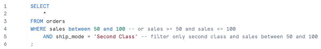
This query retrieves all columns (SELECT *) from the orders table, but restricts the results using two conditions linked by AND: the sales value must be within the defined range, and the ship mode must be 'Second Class'.
2)
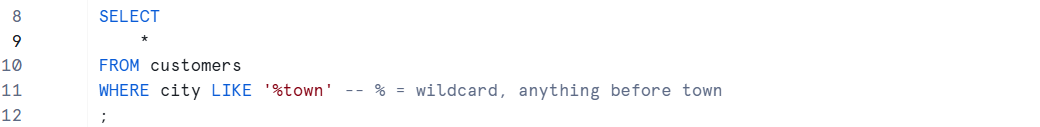
The LIKE function allows for pattern matching, typically using the percent sign (%) as a wildcard. The % is "non-greedy" and represents any sequence of zero or more characters. In this example, the query filters for rows where the city name ends with 'town'.
3)
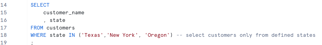
The IN function is an efficient way to filter rows where a field matches any value in a specified list, avoiding the need for multiple OR statements. This query retrieves customer names and states only for those customers in the listed states.
4)
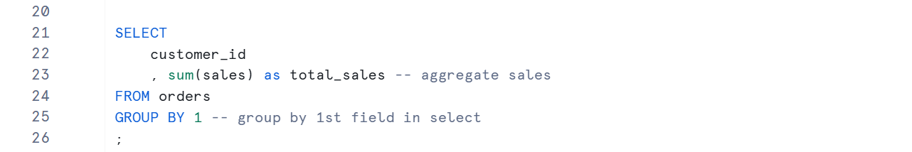
This example introduces aggregation. The SUM function aggregates sales, and the result is aliased as total_sales. Because an aggregation is used, a GROUP BY step is mandatory. The data is grouped by customer_id. Grouping by the column's position (e.g., GROUP BY 1) is a shorthand method, alternatively the column's name can be used.
5)
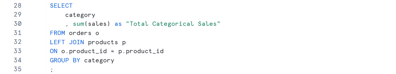
This query calculates total sales per product category, requiring data from two different tables. The LEFT JOIN is used to combine the orders table and the products table based on the common field, product_id. Tables are given aliases (o and p) to simplify calling fields within the join condition.
Note on Joins: The LEFT JOIN is one of several join types (including INNER JOIN, RIGHT JOIN, and FULL OUTER JOIN) that define the relationship between tables and determine which records are included in the final result.
6)
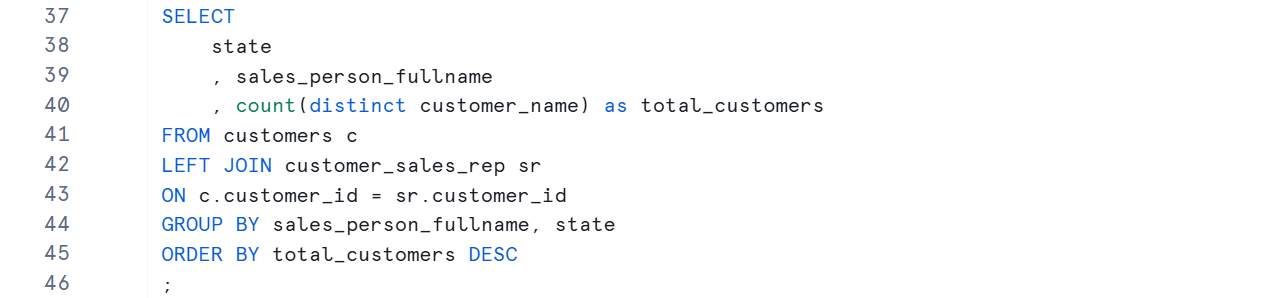
This query finds the number of unique customers assigned to each sales person. The COUNT function is combined with DISTINCT to ensure only one count per unique customer name. Finally, the ORDER BY clause sorts the result by the total number of customers in descending order (DESC).
7)
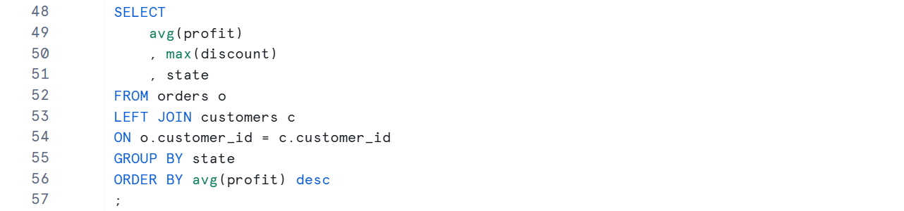
This query demonstrates the use of two different aggregate functions: AVG (average profit) and MAX (maximum discount) for each state. The results are joined across two tables and then ordered by the calculated average profit.
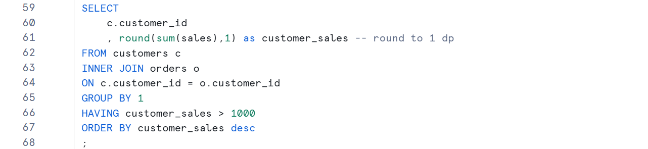
8)
This final example showcases the HAVING clause. Unlike WHERE, HAVING filters the results after the data has been grouped and aggregated. Here, the total sales per customer are calculated, and only those customers with total sales greater than 1000 are returned. The query also uses a nested ROUND function to format the output.